一个简单的神经网络代码的分析
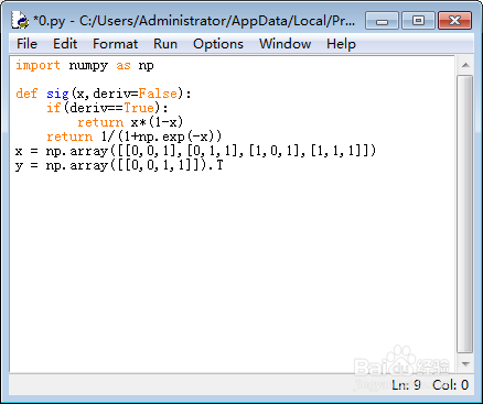
1、需要用到numpy模块:
import numpy as np
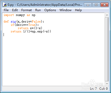
2、自定义一个sigmoid函数:
def sig(x,deriv=False):
if(deriv==True):
return x*(1-x)
return 1/(1+np.exp(-x))
3、引入训练集:
x = np.array([[0,0,1],[0,1,1],[1,0,1],[1,1,1]])
y = np.array([[0,0,1,1]]).T
x是自变量,也叫输入值;
y是因变量,也叫输出值。
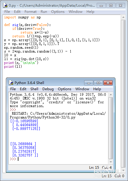
4、给出一个随机的1*3的矩阵s,并根据s构造一个1*4的矩阵l1:
np.random.seed(1)
s = 2*np.random.random((3,1)) - 1
l0 = x
l1 = sig(np.dot(l0,s))
print(s,"\n\n\n")
print(l1)
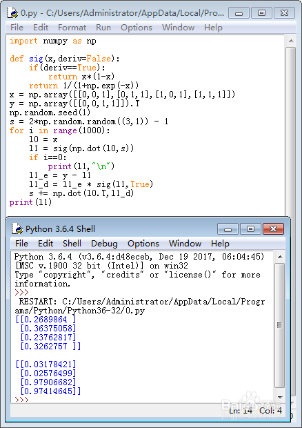
5、开始训练,使得l1逐步接近于y:
for i in range(1000):
l0 = x
l1 = sig(np.dot(l0,s))
if i==0:
print(l1,"\n")
l1_e = y - l1
l1_d = l1_e * sig(l1,True)
s += np.dot(l0.T,l1_d)
print(l1)
一开始,l1是:
[[0.2689864 ]
[0.36375058]
[0.23762817]
[0.3262757 ]]
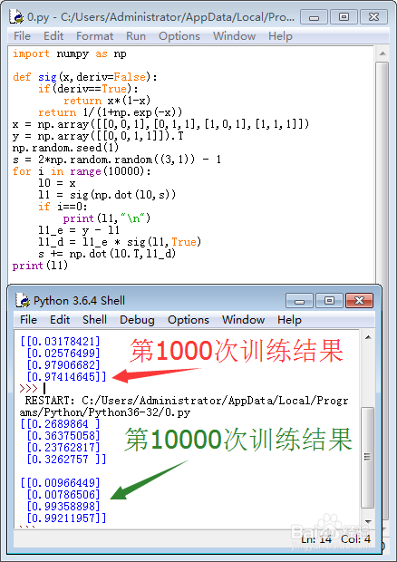
训练1000次之后,l1变成了:
[[0.03178421]
[0.02576499]
[0.97906682]
[0.97414645]]
与y已经很接近了。
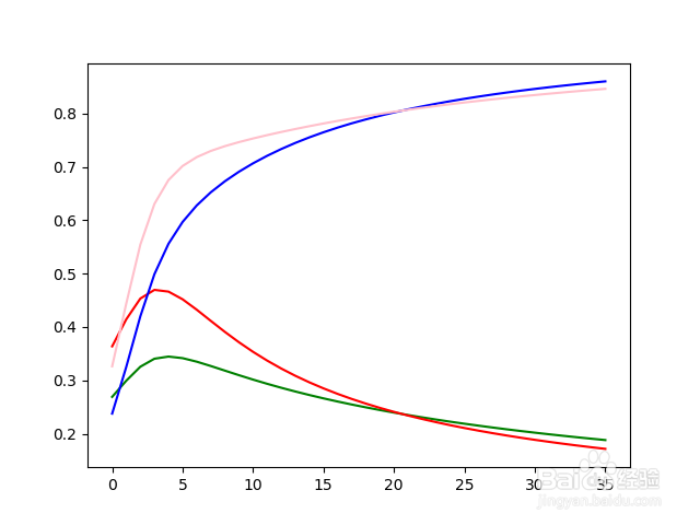
6、看看训练10000次的效果:
for i in range(10000):
l0 = x
l1 = sig(np.dot(l0,s))
if i==0:
print(l1,"\n")
l1_e = y - l1
l1_d = l1_e * sig(l1,True)
s += np.dot(l0.T,l1_d)
print(l1)
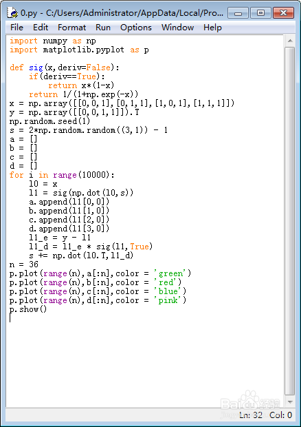
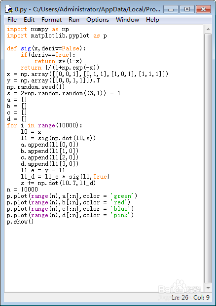
7、把训练的过程画出来,需要加载matplotlib模块:
import matplotlib.pyplot as p
然后画出折线图:
a = []
for i in range(10000):
l0 = x
l1 = sig(np.dot(l0,s))
a.append(l1[0,0])
l1_e = y - l1
l1_d = l1_e * sig(l1,True)
s += np.dot(l0.T,l1_d)
n = 10000
p.plot(range(n),a[:n],color = 'green')
p.show()
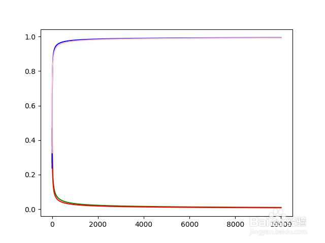
8、如果要查看前36步的训练过程,只需要把n后面的数值改为36。